Stability Relations in Forests
R. F. Mueller
March, 2000
"Sandstone, limestone and shale. These three kinds of rock characterize much of the Appalachians, with their respective properties controlling not only the topography of these ancient mountains but also their soils, ecology and biogeography."
Larry E. Morse (1988)
Forest ecology treats of development, stable characteristics and changes in forest ecosystems. Among its subjects are biochemical mechanisms of nutrient assimilation and utilization, effects of climate change, succession and genetic variation to name a few. However, central to most investigations is the question of the occurrence of a particular species in a given location at a given time. In answering this question there has properly been great emphasis on mechanisms and frequently on time rates of change. But there is another aspect of this central question that has received little systematic attention, namely factors of the mode of occurrence of species, floral and faunal, which are relatively independent of mechanisms and time rates of change, but bear on fundamental stability. An attempt is made here to identify such factors in some detail and to relate them to more familiar aspects of forest ecology, to identify an underlying structure. In order to do this it is useful to draw upon the bordering field of chemical mineralogy, a field which is also necessary to elucidate the relation of forests to their mineral substrates.
In addition to meshing directly with biology, mineral chemistry, and in particular its guiding discipline, chemical thermodynamics, provides a template for the study of biologic species in relation to their environment (Mueller, 1998). In thermodynamics the concept of equilibrium is rigorously defined as the condition under which the free energy of the system as a whole is at a minimum (Gibbs, 1957). A useful concept here also is that of metastability, in which a system is in a low, but not the lowest free energy state (or more generally, in a stable, but not the most stable state). The concept, as applicable in thermodynamics was defined by Guggenheim (1950) as follows:
"…the equilibrium of a thermodynamic system may be absolutely stable. On the other hand it may be stable compared with all states differing only infinitesimally from the given state, but unstable compared to some other state differing finitely from the given state; such states are calledmetastable." For non-thermodynamic equilibria, as applicable to forest ecology, it will be necessary to take some liberties with this definition.
One of the most elegant of the physical sciences, a strength of thermodynamics lies in its independence of specific mechanisms involved in any process. Virtually all that is required to determine stability or potential change of state (freezing, melting, chemical transformation etc.) is a knowledge of the thermal and volumetric properties of chemical phases-in this case minerals- which may be obtained with relative ease by calorimetric and related measurements. From these data the stability fields or ranges of a great variety of minerals and mineral assemblages with respect to state variables such as temperature, pressure and chemical concentrations may be obtained. These data may then be employed in the recognition and interpretation of natural equilibrium assemblages under the microscope or in the field. One can, for example, determine under what conditions substrate minerals such as calcium carbonate and silica can coexist stably or react to form other minerals. Also reactions which fix pH (1) ,oxygen concentration or other parameters can be identified. All this can be done without knowledge of the specific – often complex – mechanisms that are necessary for these reactions to occur. Furthermore, the equilibria associated with such reactions are – within certain kinetic constraints – independent of the direction from which they are approached. Thus the same equilibria may be achieved whether the system is heated from below the equilibrium temperature or cooled from above, or the pressure decreased or increased to the required value. The existence of a multitude of such paths and associated mechanisms is of no consequence to thermodynamics, which bestows a unique power of generality that is applicable to the most diverse systems of nature and undergirds virtually all industrial processes as well.
In mineral systems of metamorphic terrain, in which thermodynamic equilibrium is most closely approached as a result of pervasive recrystallization, its clearest manifestations were predicted by Ramberg (1952) and later confirmed by Kretz (1959) and Mueller (1960). These manifestations include the precise distributions of chemical elements and isotopes between coexisting minerals and consistent associations of these phases in multidimensional composition fields (phase volumes) as expressed in phase diagrams. Important parts of these diagrams are the derived phase (specific mineral) boundaries that limit the occurrence of phases in terms of state variables. Kinetic constraints on such systems were discussed by Mueller and Saxena (1977) and most recently by Kretz (1994), who has also discussed the different forms of stability. Although more difficult to determine for mineral assemblages formed under Earth surface conditions, and which form the substrates of forests, associations predicted by thermodynamic analysis are also prevalent in these cases (Garrels, 1960).
An important feature of chemical phase diagrams which also appears to be applicable to forest stability relations is the independence of equilibrium conditions in any stability field from the amounts of the various phases in a field or phase volume. Only presence or absence of phases determine a given equilibrium and these conditions are expressed in the famous Gibbs phase rule, while the relative abundance of each phase depends on the bulk composition. An extension to forest stability relations follows from a postulated analogy between biologic species and mineral phases. While there is nothing corresponding to the phase rule in biology, the number of stable plant species in a given community is clearly a function of nutrient availability, a relation analogous to the relation between the numbers of phases and chemical components.
In forests too, a condition analogous to equilibrium in mineral systems is approached rather closely. The most familiar example is the concept of the climax community. The characteristics and criteria of climax forests have been discussed by Braun (1950) and Mueller (1996). Other evidence for the attainment of some measure of equilibrium is the consistent occurrence of well-defined plant communities as implied by the applicability of such approaches as the Braun-Blanquet tabular analysis of these communities (Westhoff and van der Maarel, 1973).
Among pioneers who called attention to specific consistent relations between plants and their mineral substrates are Wherry (1916,1920), Kelley (1921), Reynolds and Potzger (1953) and Kuchler 1972). To these must also be added Braun (1950) due to her numerous incidental references to this type of relationship.
Characteristics of forest ecosystems that appear to parallel closely those of mineral assemblages are the following:
1. applicability the general criteria of equilibrium (Braun, 1950, Mueller, 1996), including those of metastability
2. faithful reflection of system chemistry as represented by substrate and atmospheric inputs
3. faithful reflection of temperature
4. occurrence of predictable associations (communities), including compatible and incompatible species
5. mutual equilibrium between all parts of the community
6. bounded and overlapping stability fields of species
7. mechanism – independent character of equilibrium
8. paramount importance of presence and absence of a species over the number of individuals of that species
9. spatial and temporal limits on equilibrium (kinetic barriers)
Although forest ecosystems may meet the general criteria of equilibrium, they
are never in thermodynamic equilibrium. (2) The reason for this is the presence of numerous gradients in state variables such as temperature and concentrations of chemical components. Furthermore, although the climax community is recognized as the best example of equilibrium, our treatment of forest stability also must include communities that have not attained climax. What such communities share with the climax communities is the continuity, if but for a short while, of the life cycle of their species. Experience teaches us that although in a stage of succession to a climax state, members of such a transitional community are compatible with the substrate, climate, light characteristics etc. Acidiphile species do not, for example, establish themselves in an alkaline environment; nor will mesic species be part of xeric or hydric communities. In general, no matter the stage of succession, species faithfully reflect habitat requirements. However species may at times become unstable or metastable as a result of changes in substrate, climate or other state variables. It has been shown, for example (Armson, 1979), that forest fires may increase the pH of shallow soil layers by several units and this effect may require decades to disappear. Thus certain acidiphile plants might become temporarily unstable or metastable. In many places in the Central Appalachians alteration of the substrate through human activities has been profound. In particular rich mesic forests originally developed on shale lost their readily erodable top soils and were replaced by far less diverse xeric and acidic types in which only a thin mor soil layer lies over bedrock.
It is likely that in addition to the obvious state variables such as temperature, chemical composition and light characteristics. in forests we must consider the duration and seasonality of suitable soil temperature and moisture. Mutual equilibrium among different parts of a community may be achieved – as it frequently is in mineral assemblages – by omnipresent media, in this case soil and atmosphere with associated nutrient cycling. One manifestation is the generally observed compatibility of shrub and herb species with the arboreal layer. Thus acidiphile herbs such as Gaultheria, Goodyera and Chimaphila characterize ericaceous oak and coniferous forests, while calciphiles such as Large-flowered Bellwort (Uvularia grandiflora), Sharplobe Hepatica (Hepatica acutiloba) and Seneca Snakeroot (Polygala senega) are associated with calciphile trees such as Black Maple (Acer nigrum), Chinquapin Oak (Quercus muehlenbergii) and Hackberry (Celtis occidentalis). A likely explanation is that both trees and herbs draw their nutrients from the same shallow root zone. Soil and rock mosses also appear to parallel these distributions, with species of Polytrichum andDicranum practically confined to acid microhabitats and those of Atrichum concentrated in more alkaline habitats, and in general acidiphile and calciphile bryophytes are well-recognized by bryologists. It seems likely that many other examples of these types of compatibilities await discovery. As in the case of mineral systems, simple observation of associated species is frequently adequate to identify equilibrium communities. Directions of change too may be recognized by certain species dropping out and being replaced by others as stability field boundaries are crossed.
Independence of mechanism signifies that, while a multiplicity of complex mechanisms enter into the establishment of most equilibria in plant communities, knowledge of these mechanisms is not necessary to identify equilibrium, the resulting stability fields and field boundaries. Such identification may be achieved by use of the general criteria of equilibrium.
The relative importance of the abundance of individuals of a species in a community and its presence or absence requires an in depth discussion of examples as presented later in this paper. Finally, as in mineral systems, the attainment of equilibrium throughout the extent of a community is limited by kinetic barriers which impose severe spatial and temporal limits on communication between different parts of the community. Such barriers universally restrict the velocities of diffusion and biochemical as well as linked inorganic chemical reactions. As in mineral systems, these barriers contribute to metastability, although this state is more complex in biologic than in purely chemical systems and is more than a thermochemical phenomenon in the former as discussed elsewhere here and earlier (Mueller, 1998). An example provided earlier (Mueller, 1998) is the successful planting of species outside their ranges, which nonetheless thrive but fail to reproduce. Recalling Guggenheims definition, such species survive slight perturbations of climate, but if destroyed by a large perturbation, can not recover because there are no viable propagules. Perhaps one of the most important consequences of these kinetic barriers is the existence of microhabitats.
To identify the stability fields of plants it is necessary to observe a broad array of occurrences and associations in the field and relate these occurrences to the substrate, topography and climate. In the short term the only reliable criterion is the presence of a species at a given site, but in the long run, consistency of absence assumes equal importance. The reason for the distinction is that presence may with great confidence be attributed to compatibility with the site in either a stable or metastable sense, while absence may result from a number of causes such as lack of seed sources, consumption by browsers and temporary exclusion by succession.
Before further analysis it is necessary to discuss specific plant communities. Figures 1 and 2 are deduced stability diagrams for some common and a few less-common woody species from the Central Appalachians. The relations shown are based on a great number of field observations by the writer as well as from the literature. However these interpretations are still very tentative and approximate. The choice of axes for these diagrams is based on both convenience and importance. Soil moisture and pH are recognized as of almost universal importance in biochemical processes (Edsall and Wyman, 1958) and their effects are readily recognizable in the field. Nutrients such as calcium, magnesium etc. are assumed to fall in the normal range except that depletion of some of these accompanies low values of pH as a result of acid leaching, and for possible other reasons. These types of relations will be touched upon later in this paper.
Nutrients play critical roles in the growth of plants, but their observed abundances in soil samples may not indicate their availability for assimilation and growth. Availability may in fact be greatly influenced by pH (Armson, 1977), and although high values of bases such as Ca and Mg are generally associated with high pH, it is difficult to correlate nutrient abundances with plant species and communities.
Both moisture and pH present serious problems of measurement and interpretation. Although pH may be determined by a variety of methods with relative ease, the meaning of some of the results may be in doubt. Furthermore, the range over many orders of magnitude of ionic concentration or activity gives an illusion of accuracy and precision that may mislead. Of necessity the positions of the field boundaries along the moisture axis are only relative, since there are few if any measurements of soil moisture – precise and reliable that they may be –which, as we shall see, bear meaningfully on stability. For example, Blackman and Ware (1982) attempted to distinguish the dependencies on soil moisture levels of Chestnut Oak (Quercus prinus) and Northern Red Oak (Q. rubra) during the growing season at two sites in the Blue Ridge Mountains. In their experiments moisture levels were determined at 15 cm depths in each case. However Metz and Douglas (1959) found that while moisture content (in this case under pine) was depleted at depths below 76 cm, higher levels were maintained at the 0 to 76 cm depths. Although a full discussion was not provided by the latter authors or by Armson (1979), in whose book they were referenced, a ready physiological explanation suggests itself. Critical to this explanation is the recognition that the fine feeder roots in the shallow zone must be kept moist to enable nutrient uptake to occur, a presumed priority function coordinated between shallow and deep roots. If this explanation is correct, the bearing on stability of measurements such as those of Blackman and Ware are thrown into doubt, although they may be important in other respects.
It is informative to compare the two axes of the figures in terms of their scales. The total range of pH observed in all Appalachian forest types is six orders of magnitude or so in ionic concentration, whereas the variation at any given site over time is usually considerably less than an order of magnitude, or one pH unit. On the other hand, moisture content is seldom observed to vary more than two orders of magnitude throughout all forest types, but may vary almost one order of magnitude at a given site over time. Thus pH is more stable at any given site than moisture content relative to total range of variability. However pH, like moisture content, may vary greatly with soil depth. Although moisture content of a soil, like pH, is here regarded as an intensive variable, it is fundamentally different from the latter. pH appears to be more a characteristic of a particular soil layer at a specific location, and is thus part of a microhabitat, although it may vary somewhat in response to weather inputs. It is frequently possible however, to obtain closely similar readings of soil pH at greatly different times and under different weather conditions. An example is soil immediately beneath mats of Polytrichum and Dicranum mosses. In contrast soil moisture may vary substantially and rapidly in response to weather inputs. Thus it is more characteristic of climate, weather and soil texture that governs retention, as illustrated once more by the data of Metz and Douglas (1959), as well as other examples provided by Armson (1977).
Additional complications arise in determining the moisture component significant to long-term plant stability. It seems reasonable, for example, that soil moisture has greater significance during the growing season than during the dormant season and that the duration and temperature of this seasonal concentration are also significant. It may even be true that the occurrence of certain species such as Chestnut Oak and Pitch Pine (Pinus rigida) are governed in part by periodic moisture deficits that preclude mesic species. Consequently soil moisture in the Figures 1 and 2 is, at this stage, based on general observations of the occurrence of species in relation to environmental factors such as topographic position and character of substrate as well as community type.
While the saturation limit of Figs. 1 and 2 is relatively easy to identify in the field, its precise location may be blurred by the velocity of water movement. Soils saturated by oxygen-rich waters may affect plants differently than those under stagnant saturation and a great number of observations may be required to clarify this situation. The dry soil limit is considerably more uncertain than the saturation limit but may tentatively be taken to lie beyond the limits of occurrence of such species as Pitch Pine and certain ericaceous shrubs such as Black Huckleberry (Gaylussacia baccata). Among such limiting occurrences may be a rock outcrop community described by Abrams and Orwig (1995) from the Shawangunk Mountains of southwestern New York State. In any case, there appears to be a strong general correlation between the ocurrence of species such as Chestnut Oak and xeric sites.
Although the locations of stability fields and their boundaries in the figures are based on field data, their general configuration is derived from principle. Using Chestnut Oak as an example, we note that as the high pH stability limit is approached we should expect diminished stability with respect to both high and low moisture as well, since the system as a whole is under stress. Consequently closed curved configurations of stability field boundaries are to be expected.
One of the firmest determinations of field boundaries is that of White Ash (Fraxinus americana) very near the saturation limit in the vicinity of pH=7. This species may be observed at the edge of a calcareous wetland in the Shenandoah Valley of Virginia (Hunsucker and Mueller, 1998), where its feeder roots lie just above the saturation zone ( here comprised of slowly moving spring water) and deeper roots penetrate it. White Ash is at this site separated by ten meters from a well-drained natural levee which supports Black Walnut (Juglans nigra), a species that cannot abide wet soils. This ash has also been observed by the writer at the edge of a swamp in calcareous terrain in east-central Wisconsin.
The intersection of the Red Maple (Acer rubrum) stability field and the acid-soil saturation limit is well-established by the common occurrence of Red Maple swamps. Similarly, the general positions of the Chinquapin Oak and Black Maple fields in the circumneutral/alkaline range of pH has been observed in the field by the writer and is well-documented in the literature (Deam, 1940; Reynolds and Potzger, 1953; Fowells, 1965)
Acid ranges in pH of some species of interest may be inferred from the data of Rawinski et al (1994) and Fleming and Moorhead (2000). (3) These are as follows:
| Species | Range | Data Points |
|
Quercus prinus | 3.4– 6.1 | 41 |
|
Acer rubrum | 3.4 – 6.7 | 50 |
|
Kalmia latifolia | 3.4 – 4.5 | 22 |
|
Fraxinus americana | 4.3 – 6.7 | 19 |
|
Acer saccharum | 4.4 – 6.7 | 9 |
These values may be compared directly with Figures 1 and 2, which were derived independently of them. However the limit of 6.7 for Acer rubrum seems high and may result from combining samples as discussed in note (3).
While no corresponding data were found for Beech (Fagus grandifolia), the range of this species was inferred from limited data in Fowells (1965) and the writer's observations. For example, the writer has observed that Beech planted on shallow soil above limestone is unstable unless the soil is acidified. To a degree a similar paucity of data exists in the case of Sugar Maple (Acer saccharum), as well as the dry soil limits of White Ash and Red Maple. However, the relative positions of the field boundaries of Red Maple, Beech, Sugar Maple and White Ash in the sequence from low to higher pH in mesic forests appears to be quite well established as shown in Figure 1.
It must also be kept in mind that the ranges of White Ash and Sugar Maple extend well into the alkaline range as is shown by a great variety of occurrences. Additionally, the range of Mountain Laurel (Kalmia latifolia) likely extends to higher pH ranges than shown in the table. For example, the writer has observed this shrub in soil with pH as high as 5.2 in a forest that included Chestnut Oak, Red Maple and White Ash.
Of some interest are the positions of the Black Oak (Quercus velutina) and Chestnut Oak fields as elucidated in calcareous terrain. There Chestnut Oak is limited to deep, leached soils or chert areas and never coexists with Chinquapin Oak. However Black Oak is clearly more widely distributed than either of the aforementioned oaks and is a familiar of very acidic terrain throughout the Appalachians as well as calcareous terrain, in which it is associated with Chinquapin Oak on limestone outcrops. It appears to be more moisture tolerant than either of the other two oaks and drops out on the driest sites where Chestnut Oak thrives.
The affinity of Great Rhododendron (Rhododendron maximum) for moist acidic sites is well known. Less familiar is the apparent extension of its stability field to calcareous sites where the writer obtained readings of pH=6.0 from highly organic soil in the root zone of this rhododendron immediately above massive limestone. However it is apparently excluded from colluvium below such outcrops, since such sites are usually subject to more alkaline solutions from above.
Although few pH data exist for Maleberry (Lyonia ligustrina), its occurrence in wet acidic sites is well documented. Ogle (1989) however provided evidence that the range of this shrub also extends to more alkaline wetlands as well, and an estimate of this range is shown in Figure 2.
It is necessary at this point to consider more of the general characteristics of the stability diagrams. Although the diagrams are at best two dimensional slices through multidimensional space, they are potentially far more complex than this since other components than those represented by the two axes are not necessarily of constant value throughout the diagrams. The stability relations shown may be – and likely are – projections on the planes shown. Thus if, as is likely, such components as calcium, magnesium, nitrogen etc. were to vary independently across the diagrams, the field boundaries should shift or be blurred from community to community. Examples of this effect are changes in pH and moisture content induced by variation of other components such as the bases calcium and magnesium. Indeed, it seems highly probable that the common decreases in pH associated with vertical leaching is precisely of this kind.A caveat also needs to be considered with regard to seedlings. It is well known that seedlings of a number of forest trees exhibit greater tolerance to shade than do mature members of the same species. Is it not possible that there is also a greater tolerance toward other growing conditions and that this is equivalent to expanded stability fields for seedlings? It is also necessary to clarify the considerable differences between diagrams such as Figures 1 and 2 and mineral stability diagrams. In the latter field boundaries mark the transformation of one or more phases into other quite different ones as a result of chemical reactions. Also, when curved, the configurations of mineral phase boundaries are usually attributable to effects such as the entropy and/or heat of transformation. In contrast, plant species do not simply transform into other species at stability field boundaries, although this may occur as part of far more complex processes. In any case, the forms of plant stability fields, as previously deduced, are likely to be related to stress factors acting on individual species.
It may be helpful to point out that although perfect equilibrium of a community such as marked, for example, by C in the figures, requires that variables of state like pH or moisture content have precisely the values shown, small deviations about these values may occur without visible change of inventoried species. It is likely that all observations of actual inferred equilibrium communities are, at best, of this type.
Complexities inherent in stability field analysis may play important roles in the interpretation of plant communities. As previously noted, the occurrence of metastable species and communities appear to be common in nature. I (Mueller, 1998) called attention to species planted outside their primary stability ranges. In nature also, a plant may seed itself or otherwise become established at locations which do not satisfy the requirements of its entire life cycle, including reproduction. Such plants may indeed flourish for a time and even produce a few offspring, but then languish and die after they exceed available living space or local living conditions. Seedlings may take root in soil that overlies chemically incompatible horizons and so perish in a season or linger for years. An example of induced incompatibility as represented by the effects of a forest fire has already been given. Another possible example noted by the writer was a mature but stunted and unhealthy-appearing Red Maple growing on a chert talus slope that is underlain by limestone. As also observed earlier ( Mueller, 1998), stable, established plants such as Hemlock (Tsuga canadensis) may, by their influence on soil over time by foliage drop, destabilize other species in the vicinity. The effect of plant toxins such as those produced by Black Walnut are well known ( Fowells, 1965). Familiarity with stability field analysis enables the observer to rapidly assess the potential for such relations in the field. Genetic variability however introduces less obvious effects, as for example, when an ecotype of a species invades terrain unusual for that species.
Diagrams such as Figures 1 and 2 may also aid in the interpretation of the relative abundance of individuals of a species in the canopy of a given stand of trees. In general it might be expected that the number of individuals of a species might be relatively low, as at position C in the figures, where a number of other species are stable. In contrast, stability field positions that fall in extreme arboreal ranges, as those of Red Maple and White Ash in proximity to the water saturation limit and Chestnut Oak at its dry soil limit, would be expected to have but few species in a stand. An extreme example is the tropical forest, in which so many species are stable that the densities of all species are low. These examples are quite obvious, but many other, more subtle relations of the sort, might be cited. A corollary of these relations is that the number of individuals of a given species in a stand is not necessarily indicative of its relative stability. An example of a species that shows this type of behavior in a number of forest types is White Ash. Low densities of certain species may result from competition or a variety of events or processes, and not at all from instability with respect to substrate or climate, although such factors as light character may be involved.
Additional Applications and Summary
Stability field analysis serves as the basis for a number of ecological investigations in forests. It provides baseline standards of forest type and species occurrences for studies of disturbances and succession and is mandatory for a comprehensive interpretation of forest stands.
Stands of trees, recognized as such, frequently number in the hundreds of canopy individuals and extend over several to many acres of terrain with greatly varying topography, substrate and even microclimate. In many investigations terrain showing conspicuous variation of this type is avoided, or if not conspicuous, the variation may be disregarded. However, to see most clearly the effect of substrate, topography and microclimate on forest type and species distributions, it is desirable to observe as broad a range of conditions and habitats as possible. To date few examples of such comprehensive studies exist in the literature. One of the most informative and generally superior of such studies, even after the long lapse of time since its execution, is Braun's ( 1950) Deciduous Forests of Eastern North America. Of particular utility are the extensive tabulations of stand compositions from her mixed mesophite and western mesophite regions, since these regions encompass great variations in geology and topography and thus capture the most striking examples of floral response.
Braun's study sites were selected with such great care that even stand scale data reflect the strong relations between vegetation and substrate, However, close examination also enables one to discern a number of microhabitat influences in these data as well. Most of the stands she tabulated were located on rugged slopes or in ravines of the Cumberland Plateau or similar highly dissected areas to the west, where two very dissimilar rock types, limestone and sandstone, are frequently juxtaposed. Trees that stand out as indicator species are Red Maple, Beech, Chestnut Oak (all acidiphile) and Chinquapin Oak (calciphile). Her studies show the incompatibility of Beech and limestone substrate as exemplified by the Inner Bluegrass region of Kentucky and the limestone terrain of the Knobs Border region. The mutual antipathy of Chinquapin Oak and Beech, Red Maple and Chestnut Oak in the Tennessee Cliff Section of the mixed mesophyte region is displayed in her Table 18. Other examples of such exclusions could be cited. However, her data also contain more ambiguous but still interesting examples in her tables 19, 21, 22, 25. 27 and 29, which represent large stands, all rich in Beech,with small quantities of Chinquapin Oak. It is likely that this apparent contradiction results from isolated patches of calcareous terrain, perhaps in the form of limestone outcrops. As we have seen, Chinquapin Oak appears to be virtually confined to such sites, which might be expected to have only scattered occurrences in the deep mull soils of the colluvial slopes and ravines she inventoried. A similar example is found in a variety of unusual calcareous communities inventoried by the Virginia Natural Heritage Program (Fleming, 1999). In their 400 square meter study plots, acidiphile species occasionally were recorded in dominantly calciphile communities, and soil pH showed variation in the plots as well. These examples illustrate a general problem with inventories of large stands or study plots considered as units even when the inventories are of the high quality as these are. The same caution also applies to bryophytes and fungi, all of which can, in stand scale inventories, give rise to contradictions that may be resolved by considering microhabitats. In such inventories communities do not correspond to equilibrium points but to areas (really volumes in multidimensional space).
There is also a parallel between the ranges of species and their local occurrence and microhabitats. Species that ascend highest in mountains generally range farthest north. More subtly, species which are associated with alkaline or calcareous sites in the east, are more likely to range farthest west (Fowells, 1965) since there is a general increase in alkalinity from east to west. The latter effect is however complicated by a parallel decrease in moisture which also restricts some species. There are of course contradictions to these trends, in particular with respect to elevational effects. There is a considerable number of plants that ascend to high elevations, but do not range far north. It is possible that these are ecotypes and may be responding to light intensity or other factors.
Most investigations in forest ecology appear to be conducted on a stand scale. In some cases, such as dendroecological studies, this is mandatory, since at a minimum only stands can provide the range of species and tree ages required. However, there are many investigations which have, at least by implication, as their major objectives stability relations, and here, as indicated in the examples cited above, the stand scale is too coarse to discern many processes at work. Frequently data from different stands of a forest type are combined, and only average values presented. In some cases important soil indicators such as pH or chemical concentrations are handled in this way even when the combined stands occur on substrates ranging from siliceous to calcareous. The existence of valuable data of this type may be mentioned but not presented. In the resulting statistical analysis of many studies, correlations are sought from combined data instead of recording actual observable correlations between species individuals and specific substrate locations. In many studies much attention is also given to precise determinations of the number of individuals of saplings, seedlings and herbaceous species in a stand without any discernable purpose. As previously mentioned, by analogy with mineral systems, numbers of individuals may not be nearly as significant as the presence, absence or locations of the species in question when stability is a consideration. In any case, arbitrarily distinguishing "seedlings" from "saplings" solely by size, as is conventional, is likely to be meaningless. An example of an interesting and productive type of observation was that of Carr (1939) who noted that in the Magnolia Swamp of Augusta County, Virginia, acid – loving species were rooted on hummocks of humus, whereas calciphiles had their roots in positions that were in contact with upwelling groundwater. In each case, soil associated with calciphiles had pH=7.0, while soil associated with acidiphiles ranged between pH= 4.0 and 5.0. In calling attention to this observation, Fleming (1999) cited possible similar relations in another wetland. The writer has also observed such microhabitats in wetlands as indicated by juxtaposed contrasting flora and they are very prevalent in upland forests, where they may be induced by vertical acid leaching, proximity to contrasting strata or other effects. In some instances a variation in pH of almost two units over a distance of a meter have been observed. An interesting situation arises when, as on some alluvial deposits, there is an intimate mix of a variety of rock types, in particular, sandstones and limestones, and which, as observed by the writer, have given rise to closely juxtaposed acidiphile and calciphile plants. It has been shown ( Korner,1999) that plant roots will concentrate in soil volumes favoring growth, such as those artificially fertilized, and it appears reasonable that in rock mixtures each plant might seek out with its roots the rock or soil appropriate to its species. To summarize, the most ecologically significant data bearing on stability of species and forest types may be obtained from microhabitats and observation of the widest possible range of habitats and occurrences of species.
It also seems necessary to revisit the concept of the climax forest in relation to types of climax defined in the current literature. While relatively stable old growth mixed mesophyte forest is universally regarded as a "climatic" climax in the Appalachians, dry oak forest of ridges and a variety of other forest types may be regarded as either "physiographic" or "edaphic" climaxes. It is curious that the inherent contradiction in this terminology does not seem to have been widely recognized. This contradiction may be seen by considering that the mixed mesophyte forest type is a product of rich colluvial slopes and ravines as well as a humid climate, whereas the so-called physiographic or edaphic climax is the result of other topographic and substrate conditions under a similar or somewhat different climate. However since there are many gradations between all these forest types, we have no a priori reason to believe that one or the other is more or less a product of either climate, topography or substrate. As I concluded earlier (Mueller,1998), all three as well as biologic factors contribute not only to the climax stage but to all forests at every stage of development.
In addition to introducing a new perspective, stability field analysis creates greatly expanded opportunities for research, particularly in field classification of species and forest types, but also in the detailed correlation of chemical, physical and climatic data with species distributions. Although its application is here limited to the Central Appalachian forests, the generality of its approach indicates that it should be applicable to forest and terrestrial ecosystems everywhere.
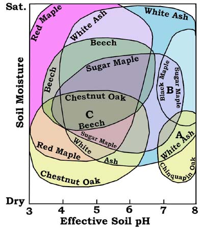
Fig. 1-Tentative overlapping tree stability fields with resulting associations (A, B, C) as a function of field position. Concept by RF Mueller, graphic by the Gus.
B: Black Maple-Sugar Maple-White Ash
C: Chestnut Oak-White Ash-Sugar Maple-Red Maple-Beech